- The CAFE rollback changes the long-term fuel-demand outlook, while both central modeling paths still show consumption declining.
- NHTSA’s cumulative difference of 122 billion gasoline-equivalent gallons comes from a constrained regulatory model, not a forecast of tanker loads.
- For petroleum carriers, customer retention, terminal access and delivery productivity will determine the commercial outcome.

A Bradley fuel tanker connected to delivery hoses at a Commerce City, Colorado, gas station in April 2016. (Photo: Xnatedawgx/Wikimedia Commons; CC BY-SA 4.0)
A gasoline demand reset is taking shape in Washington, with consequences that could reach well beyond automobile factories. The Trump administration’s September 28 release of revised Corporate Average Fuel Economy standards changes the policy assumptions behind the cars and pickups that consume the fuel petroleum carriers deliver.
For tank fleets, the central question is how much gasoline business remains over the life of a customer contract, tractor or trailer. A slower decline could support more delivery work than under the previous-rule scenario, even while total consumption continues to fall.
That distinction matters. The rule does not establish how many additional tanker loads carriers will haul. Its commercial significance lies in the planning horizon: the durability of retail demand, the use of distribution assets and the competition to serve the gallons that remain.


This development concerns passenger cars and light trucks. It is separate from NHTSA’s review of heavy-truck fuel-economy authority, which addresses the equipment used to move freight. Here, the connection runs through the vehicles buying the delivered product.
A slower decline can preserve delivery work without producing a growing national gasoline market.What the gasoline demand reset changes
NHTSA’s final rule, signed September 25, recalibrates standards for model years 2022–2031. The agency’s posted version specifies an effective date 60 days after Federal Register publication; the September 28 announcement itself is not the effective date.
The agency projects an industrywide average requirement of about 34.9 mpg for model year 2031. It also ends inter-manufacturer credit trading beginning with model year 2028 and changes passenger-car and light-truck classifications beginning with model year 2030.
These are manufacturer compliance provisions. The 34.9-mpg figure is not a prediction that the entire existing U.S. vehicle fleet will average that mileage in 2031, nor a fuel-economy guarantee for an individual vehicle.
The business effect depends on what automakers build, what motorists buy and how quickly those purchases replace vehicles already in service. A revised standard changes one influence on those decisions; it does not specify the future sales mix at every dealership or gasoline demand in every county.
The near-term outlook still points downward
Love’s Freightliner tanker truck in southern Oklahoma. (Photo: Greg Goebel/Wikimedia Commons; CC BY-SA 2.0)
EIA’s September Short-Term Energy Outlook puts U.S. motor gasoline consumption at 8.91 million barrels per day in 2025, 8.76 million in 2026, and 8.75 million in 2027. Published September 9 using information finalized September 3, that outlook predates the CAFE announcement.
Those figures provide a near-term reference, not a post-rule forecast. They cannot be revised by simply adding a long-range NHTSA scenario difference. The agencies’ calculations answer different questions, use different assumptions, and cover different measures of fuel use.
EIA explained in April that automotive design, development, and production cycles often take five to seven years, limiting the immediate effect of policy changes. It also identified efficiency gains and hybrid adoption as factors influencing consumption.
The operational implication is a lag between an announcement in Washington and a change at the loading rack. Existing vehicles still require fuel, while replacement vehicles gradually change the fleet’s fuel consumption per mile. Meanwhile, employment, commuting, travel and household spending can move local sales before a revised vehicle standard becomes visible in the fleet.
A carrier serving a growing retail customer could gain volume during that transition. Another could lose business where stores close, or motorists buy less fuel. Neither outcome, by itself, would establish whether the national regulatory model was right.
Reading the fuel-consumption model correctly
Table V-10 of NHTSA’s final rule estimates approximately 122 billion additional gasoline-equivalent gallons cumulatively over calendar years 2024–2050 under its selected alternative. NHTSA reports the increase as 4.6% above its no-action baseline.
The selected annual values illustrate when the difference develops. These are modeled light-duty liquid-fuel consumption totals, expressed in billions of gasoline-equivalent gallons.
| Calendar year | No-action scenario | Final-rule scenario | Additional use vs. no action |
|---|---|---|---|
| 2031 | 108.6 | 110.9 | 2.3 |
| 2040 | 86.0 | 92.5 | 6.5 |
| 2050 | 75.8 | 83.1 | 7.3 |
Both columns decline. In this model, the rollback preserves consumption relative to the alternative; it does not reverse the downward direction in these selected years.
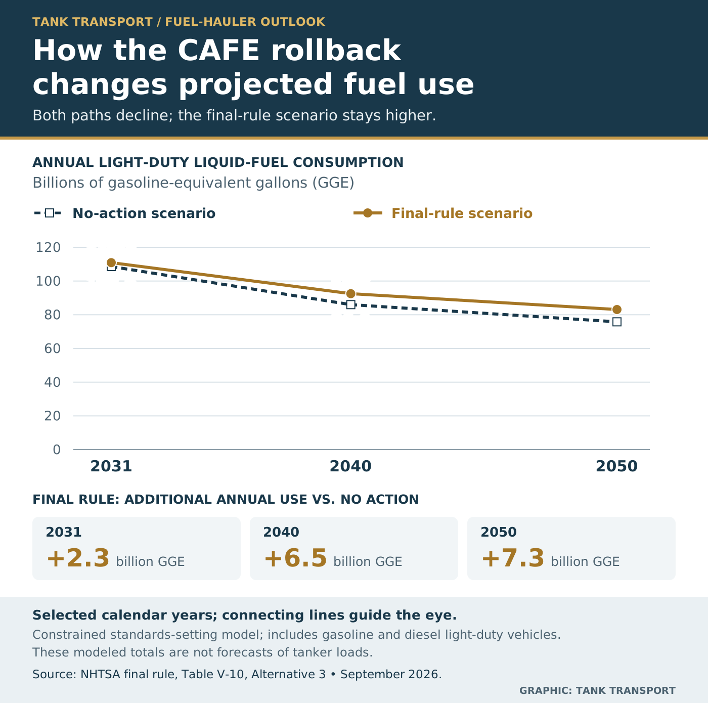
NHTSA’s model projects declining light-duty fuel consumption under both scenarios, with the final rule producing higher annual use than the no-action baseline. Values are billions of gasoline-equivalent gallons. (Graphic: Tank Transport; source: NHTSA, Table V-10, Alternative 3)
The scale warrants attention because fuel-distribution investments can outlast several vehicle-model cycles. But the difference between scenarios is useful only when its boundaries remain attached to the numbers.
Why 122 billion gallons is not a freight forecast

A Sunoco fuel tanker at Woodhaven Boulevard and Metropolitan Avenue in Queens, New York. (Photo: Tdorante10/Wikimedia Commons; CC BY-SA 4.0)
NHTSA’s environmental statement explains that its standards-setting analysis sets aside potential compliance credits and certain alternative-fuel technologies under the governing statute. Its separate environmental analysis allows broader manufacturer responses, including electrified powertrains. Those analyses have different scopes and cannot be combined into one demand series.
NHTSA’s final regulatory impact analysis describes a no-action case that evaluates existing standards with the current analytical framework. It is not an unchanged forecast copied from the previous rulemaking. The comparison measures the effect of alternatives within a model.
The long-range comparison holds model-year 2031 standards in place afterward and assumes manufacturers make practicable efforts to comply despite a statutory $0 CAFE civil penalty rate. Future policy and manufacturer behavior could depart from those assumptions.
Gasoline-equivalent gallons add another boundary: they express energy on a common basis. The central liquid-fuel analysis includes gasoline and diesel use by light-duty vehicles. It is not a count of finished gasoline gallons scheduled for delivery to service stations.
Dividing the cumulative number by an assumed tanker capacity would therefore create false precision. Such a calculation would still need to identify the actual fuel, year, consuming location, delivery channel, load size, and carrier serving each movement.
A national consumption scenario becomes a hauling opportunity only when it connects to a customer, a terminal and a delivery requirement.The model is most useful for testing assumptions. If a fleet’s long-range plan assumed rapidly disappearing gasoline business, the policy change warrants another look. It does not establish a revised demand forecast for that fleet.
The policy trade-off extends beyond carrier revenue
DOT presents the reset as an affordability measure, estimating a $1,300 reduction in the average cost of a new vehicle. That is the administration’s estimate, not an observed reduction in transaction prices following the announcement.
NHTSA’s separate environmental analysis projects higher fuel consumption and carbon dioxide emissions relative to its no-action case. The potential preservation of petroleum-delivery business therefore sits alongside fuel-use and environmental costs.
For a carrier, the commercial question is narrower than the policy debate: whether its customers will need dependable gasoline deliveries for longer, and on what terms. Answering that question does not require treating additional fuel consumption as an unqualified economic benefit or assuming every projected policy saving will materialize.
How national gallons become tanker work
EIA describes a distribution chain in which most gasoline moves from refineries through pipelines to storage terminals near consuming areas. Ethanol and other components are blended into finished fuel, and tanker trucks handle deliveries to retail stations. Different retail brands can obtain supply from the same terminal.
That network explains why the gasoline demand reset has several possible commercial outcomes. More persistent demand could help retain activity at an existing rack. It could also be concentrated among customers supplied from a different terminal or carried by a competing fleet.
The gallon is only the beginning of the transport calculation. A nearby high-volume store and a distant low-volume outlet can require very different amounts of truck time to receive the same aggregate quantity. Compartment requirements, delivery windows, unloading time, and the return trip further separate fuel demand from productive capacity.
Fixed costs make the slope matter
Sunoco’s 2025 annual filing directly identifies fuel-efficiency standards as a demand risk. The company says some distribution expenses are fixed, so falling gallons may not bring proportional cost reductions and can pressure margins.
The filing also says sustained demand losses can affect pipeline throughput and terminal storage after existing throughput and deficiency agreements expire. Sunoco distributes fuel using its own fleet alongside third-party and affiliated carriers.
For a petroleum carrier, the analogous question is how much dependable work remains to support the assets and people assigned to an account. If a slower decline keeps an existing shift productive, it can have value without requiring another truck.
That distinction changes the investment discussion. Preserving utilization may justify maintaining reliable equipment or renewing a customer commitment. Expansion requires another layer of evidence: enough additional, serviceable work to cover the added capacity.
A customer’s contractual promise also differs from the physical delivery pattern. A minimum commitment can allocate commercial risk, but dispatch still needs workable routes, loading access, and delivery windows. The strongest business case connects both sides.
Ownership changes can outweigh the national trend
Sunoco’s second-quarter 2026 filing illustrates another complication. It reported 4.125 billion motor-fuel gallons sold, compared with 2.188 billion a year earlier, and attributed the increase primarily to the Parkland acquisition. Those are companywide motor-fuel figures, not a measure of organic U.S. gasoline-demand growth.
A distributor can expand while the overall market softens. A carrier can gain an account because ownership changes, or lose it because the buyer combines networks. In either case, the immediate commercial event may be customer strategy rather than a national fuel-consumption change.
Tank Transport’s coverage of the Sunoco–Offen fuel-network agreement and ARKO’s USPP transaction and terminal network provides related context for how distribution assets and customer relationships enter acquisition decisions.
The question for independent carriers is where outsourced transportation fits after those networks change. A broader customer footprint may offer more opportunities, but an integrated private fleet or revised procurement strategy could capture them. The CAFE rule does not choose that outcome.
Company growth, national demand and an individual carrier’s workload are three different measures.Regional supply still shapes the route

Petroleum storage tanks, docks and rail infrastructure along Houston’s industrial waterway in April 2015. (Photo: formulanone/Wikimedia Commons; CC BY-SA 2.0)
EIA’s analysis of California highlights limited connections to other refining centers and specialized gasoline requirements. Those structural conditions help explain why a national average cannot describe every regional supply system.
For hauling, the relevant geography is even more detailed: the terminal a customer can use, the route from that terminal, and the hours available to complete deliveries. A supply change can lengthen a haul even when customer gallons are unchanged. A new source closer to the customer can do the reverse.
This produces a second planning variable alongside volume: the amount of transport work required per delivered gallon. More miles or waiting time may require additional capacity while weakening productivity. A rise in truck hours is not automatically a rise in attractive business.
A national demand model cannot identify those local changes. Terminal activity, customer nominations and actual route performance remain the evidence that connects the broader outlook to fleet economics.
What belongs in a fuel fleet’s investment case
The useful response to a changed long-term outlook is a more explicit business case. The relevant evidence falls into three horizons: work already committed, business under negotiation, and future demand scenarios.
Committed work can support near-term staffing and equipment decisions when you understand its duration, pricing, and delivery requirements. Negotiated work introduces customer and execution risk. A national scenario supplies background for both, but cannot substitute for either.
This framework also distinguishes replacement from expansion. Replacing unreliable equipment may protect an existing service obligation even in a declining market. Adding net capacity requires a credible source of additional utilization.
Four operating measures that connect the outlook to the fleet
Customer gallons and contract duration. Start with account-level demand across comparable periods, adjusted for outlets added, lost, or acquired. Contract length and renewal timing show how much of that volume is actually secured.
Delivered gallons per truck-hour. This measure connects volume to loading, driving, waiting, and unloading time. It helps distinguish a useful increase in demand from a workload that consumes more capacity without a matching revenue improvement.
Loaded and empty mileage. Changes in supply points can alter the cost of serving existing customers. A longer replenishment route may create more miles to bill, but the commercial result depends on the rate structure and the availability of drivers and equipment.
Contribution after service costs. Additional gallons have limited investment value when the associated work fails to cover its costs. Pricing, accessorial treatment, and schedule reliability belong alongside volume in any expansion assessment.
A simple illustration shows why the measures belong together. Suppose an account requires 100 truck-hours per week to deliver its regular volume. If a supply-point change raises the requirement to 115 hours while gallons stay constant, the account needs 15% more truck time. Nothing in that example represents demand growth.
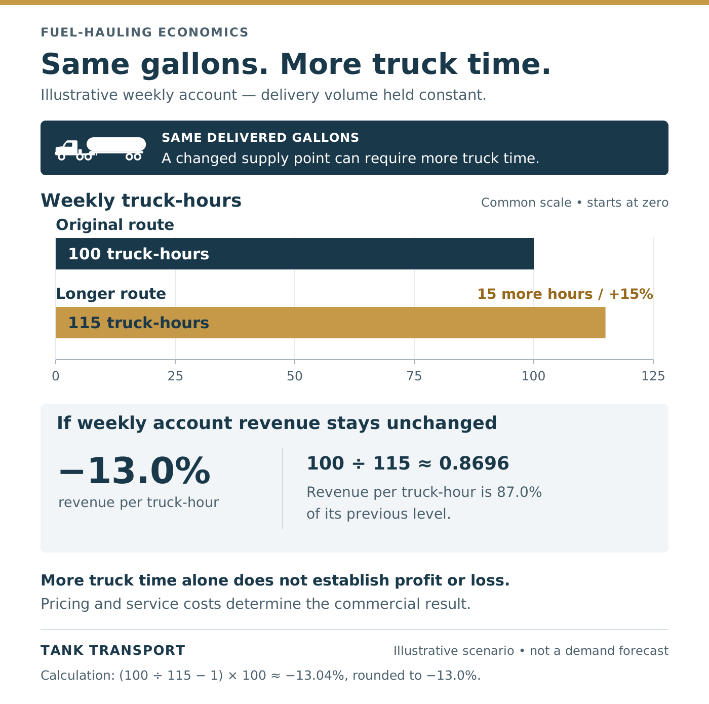
Delivering the same fuel volume with 15% more truck time reduces revenue per truck-hour by approximately 13% if weekly account revenue remains unchanged. Illustrative example. (Graphic: Tank Transport)
If compensation stays unchanged, revenue per truck-hour falls. If the contract properly recognizes the extra work, the account may remain attractive. If additional hours displace better-paying deliveries, the apparent opportunity could still weaken the fleet’s overall results. These are hypothetical outcomes, but the calculation identifies what a demand headline leaves unanswered.
The reverse also matters. Better loading access or a closer terminal can allow existing equipment to handle more gallons. A carrier may capture additional sales without buying another trailer, preserving financial flexibility if the broader market later weakens.
Which vehicles are actually replacing the local fleet?
DOE’s Alternative Fuels Data Center publishes state registration counts that separate gasoline vehicles, diesel vehicles, conventional hybrids, plug-in hybrids, and battery-electric vehicles. The distinctions matter because electrification does not describe one uniform effect on liquid-fuel use.
A conventional hybrid still purchases fuel. Plug-in hybrids’ gasoline use depends partly on charging and driving patterns. Registration counts also describe vehicles, not their annual mileage or the stores where their drivers buy gasoline.
Consequently, state fleet data can help frame a regional scenario but cannot determine a carrier’s sales forecast. Customer sell-through and delivery records provide the closer commercial evidence.
The investment case strengthens when national scenarios, local vehicle trends and customer delivery records point in the same direction.A stronger investment signal would combine several observations: sustained customer sell-through, a contract covering the proposed equipment commitment, and delivery records showing that existing capacity is consistently occupied. A policy announcement can prompt that review; operating evidence determines the outcome.
A weaker signal would be one unusually busy period, a temporary terminal disruption, or gallons gained through a short-lived reassignment. Such work may generate revenue, but its duration matters when matching it to a multiyear equipment obligation.
This also creates a practical distinction between preserving options and committing capital. Maintaining serviceable equipment, documenting terminal alternatives, and retaining customer relationships can keep a fleet positioned for several demand paths. A permanent capacity increase narrows those options unless dependable work follows.
The gasoline demand reset gives petroleum carriers a reason to revisit how quickly they expect their market to change. The strongest opportunity may be additional years of productive service from an existing network. Whether that becomes a durable advantage will depend on customer commitments and execution at the rack, on the road, and at the delivery point.
Gasoline demand reset: Key Developments
- Status: The final rule has been released, with effectiveness tied to Federal Register publication.
- Direction: The selected consumption scenarios remain downward.
- Scale: The cumulative modeling difference is substantial, but its units and assumptions limit direct conclusions about freight.
- Timing: Vehicle replacement and production cycles separate policy announcements from delivery effects.
- Commercial exposure: Customer ownership, private-fleet decisions, and terminal geography influence which carriers serve the market.
- Investment test: Account-level commitments and route productivity provide stronger evidence for new capacity than national totals alone.
- Unresolved: The rule’s effect on carrier equipment orders, hiring and capital spending remains unknown.
Fuel-Economy, Demand and Distribution Sources
- DOT’s September 28 announcement presents the administration’s rationale and projected vehicle-cost savings.
- NHTSA’s CAFE rulemaking page summarizes the compliance changes and links the supporting documents.
- The signed final rule, particularly Table V-10 on page 702, provides the central liquid-fuel scenario comparison and effective-date language.
- NHTSA’s final supplemental environmental impact statement, Section 2.3.1, explains the constrained and unconstrained analyses.
- The final regulatory impact analysis (Chapters 3 and 8) details the baseline and compliance modeling.
- The environmental statement summary describes the separate emissions assessment.
- EIA’s September 2026 outlook, Table 4a, supplies the near-term gasoline-consumption figures.
- EIA’s analysis of efficiency and gasoline consumption explains vehicle turnover and automotive production-cycle timing.
- EIA’s gasoline-distribution overview traces supply through terminals and retail delivery.
- Sunoco’s 2025 annual filing describes demand risks, fixed costs, and transportation arrangements.
- Sunoco’s second-quarter 2026 filing distinguishes acquisition-driven volume growth from underlying market demand.
- EIA’s California supply analysis explains regional constraints and fuel specifications.
- DOE’s state vehicle-registration data provide a regional view of powertrain composition.